
 EN
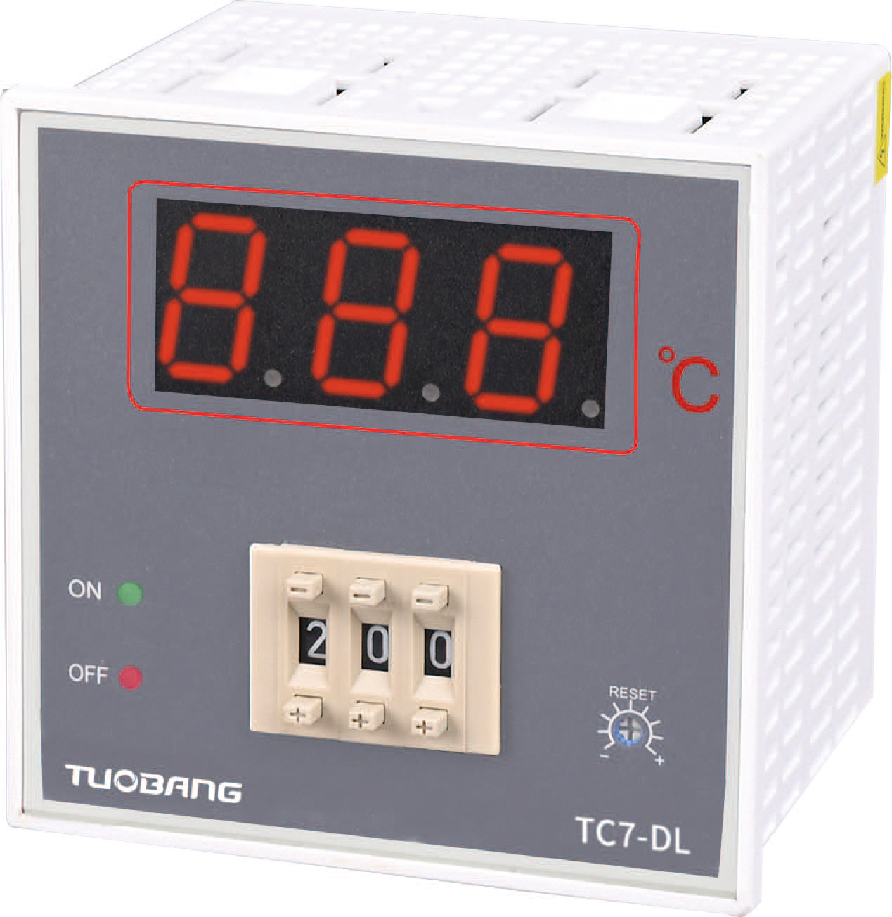
When autotuning is not enough
Most modern temperature controllers come with an autotuning function. Push a button or set a parameter, and the controller runs a test sequence to characterize the process and calculate PID values. When it works, it works well. When it does not work, the results can be worse than no tuning at all.
Autotuning struggles in specific situations. Processes with long dead times, where the sensor is far from the heater and there is a significant delay between a change in heater output and a change in the measured temperature, confuse the autotuning algorithm. Processes with noisy sensor signals cause the autotuner to misinterpret normal fluctuation as a process response. Processes where the operating conditions change significantly between startup and steady state, such as a batch reactor that goes from cold to hot, cannot be captured by a single autotuning run.
Manual tuning is slower and requires more judgment. It is also the only option when the controller is in a critical process and a failed autotune is not acceptable.
Preparations before touching a single parameter
Before adjusting anything, the process should be at a representative operating condition. Tuning at room temperature and then running at production temperature is a recipe for disappointment, because the thermal behavior of most materials changes with temperature. A heater that is adequate at 100 degrees may be marginal at 300 degrees, and the controller settings that worked at low temperature will be wrong at high temperature.
The sensor position matters too. If the sensor is not in a location that represents the temperature that actually matters, no amount of tuning will fix the mismatch. Checking sensor placement is a prerequisite, not an optional step.
The controller should be in manual mode with the output at a level that holds the process at or near the target temperature. This establishes a baseline. From that baseline, the effect of each parameter change can be observed.
A step-by-step approach for heating loops
The most reliable manual tuning procedure for a heating loop starts by zeroing out the integral and derivative terms. With integral and derivative at zero, the controller behaves as a pure proportional controller. The proportional band should be set wide, so the controller responds gently. Then the proportional band is narrowed in steps, allowing the process to settle between each adjustment.
The goal at this stage is to find the proportional band at which the temperature just begins to oscillate. That is the critical proportional band. Once found, the band is widened by a factor of roughly two to three. This gives a stable response with a modest steady-state offset.
Next, the integral term is introduced. It should start at a value that produces a very slow correction, meaning a long integral time. The integral time is then shortened in steps, again allowing the process to settle between adjustments. The goal is the shortest integral time that eliminates the steady-state offset without introducing oscillation.
The derivative term is added last, if it is added at all. It should start at a very small value. If the approach to setpoint still shows overshoot after proportional and integral are well tuned, increasing the derivative term slightly can help. If the temperature becomes erratic or the response becomes sluggish, the derivative term is too large.
| Step | Action | What to Watch For |
|---|---|---|
| 1 | Zero I and D, set wide P band | Stable temperature with offset |
| 2 | Narrow P band gradually | Oscillation threshold (critical band) |
| 3 | Widen P band to 2-3x critical | Stable response, acceptable offset |
| 4 | Introduce I, start with long time | Offset begins to shrink |
| 5 | Shorten I time gradually | Offset eliminated, no oscillation |
| 6 | Add small D if needed | Overshoot reduced, no erratic output |
The step response test and what it reveals
An alternative to the trial-and-error approach is a step response test. With the controller in manual mode and the process at steady state, the output is increased by a fixed amount, say ten percent. The temperature response is recorded. The shape of that response reveals the process characteristics: the dead time before the temperature starts to rise, the maximum rate of rise, and the time it takes to reach a new steady state.
From the step response, PID parameters can be estimated using rules such as the Ziegler-Nichols open-loop method or the Cohen-Coon method. These rules provide starting points that are usually in the right neighborhood. The step response test has the advantage of being done in open loop, which means the controller is not fighting the process while the test is running.
The disadvantage is that the step response test assumes the process is linear and that the step size is small enough not to excite nonlinearities. In real thermal systems, both assumptions are approximations.
The common mistakes that waste hours
One of the most frequent errors is tuning with the derivative term active from the start. The derivative term responds to the rate of change of temperature, and if it is set before the proportional and integral terms are reasonably tuned, it amplifies every sensor noise and makes the process look unstable when it is not.
Another common mistake is adjusting multiple parameters at once. When the proportional band and the integral time are changed simultaneously, it is impossible to tell which change caused the observed effect. One parameter at a time, with enough settling time between adjustments, is slower in the short run but faster in the long run.
A third mistake is tuning at a setpoint that is not representative of normal operation. The PID parameters that work well for a setpoint of 80 degrees may not work well for 200 degrees. If the process runs at different setpoints, the controller should be tuned at the most critical one, or a gain scheduling approach should be used.
In a food processing plant, a pasteurization tunnel had been autotuned at startup with cold water flowing through the system. The autotune produced aggressive parameters that were fine for the cold start but caused the temperature to overshoot by more than fifteen degrees when the tunnel was loaded with product. Manual tuning at production temperature with product in the tunnel produced parameters that held the temperature within two degrees.
The practical reality of manual tuning in production
Manual tuning in a production environment is always a compromise. Taking a process offline to tune it properly costs money. Tuning while the process is running risks producing off-spec material. The practical approach is to identify a window when the process can be run at a reduced rate or with a less critical product, and use that window to establish the basic parameters. Fine adjustments can then be made during normal operation when the process is stable.
It also helps to record what was done. The next time the process needs tuning, having a record of the parameters that worked and the reasoning behind them saves a lot of time.
Suosite’s temperature controllers provide both manual tuning access and autotuning functions, and the parameter conventions are consistent across the product family. That consistency matters when a panel builder is commissioning multiple loops on the same machine and wants the tuning experience from one loop to transfer directly to the next.